Weekly Report [4]

Jinning, 08/07/2018

Clip experiment on large dataset

Got the result of Clipping with \(\min\{\frac{1}{p}, c\}\). This result is trained and tested on large dataset.

Loss function used (weighted BCE loss):

\[ -\min\{\frac{1}{p}~,~c\}\left[ y \cdot \log \sigma(x) + (1 - y) \cdot \log (1 - \sigma(x)) \right] \]

\(c\in\)[1, 2, 5, 10, 15, 20, 30, 50, 100, 150, 200, 250, 300, 350, 400, 450, 500, 550].

In the training set, the value of \(\frac{1}{p}\) varies among \([1, 2917566]\). Its average is \(114.57\).

Distribution of inverse propensity

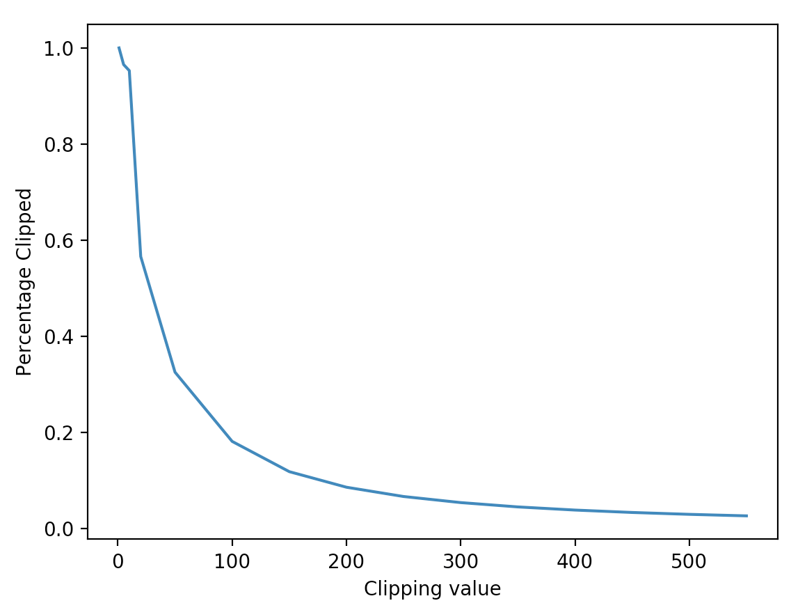
In order to survey the distribution of \(\frac{1}{p}\) , the following diagram show the percentage of \(\frac{1}{p}\) larger than given \(c\) (which is clipped):

[100.00%] 14175476 in 14175476 larger than 1
[96.52%] 13682662 in 14175476 larger than 5
[95.78%] 13577934 in 14175476 larger than 10
[56.56%] 8018069 in 14175476 larger than 20
[45.15%] 6400434 in 14175476 larger than 30
[32.50%] 4606483 in 14175476 larger than 50
[18.09%] 2564603 in 14175476 larger than 100
[11.79%] 1671481 in 14175476 larger than 150
[8.55%] 1212462 in 14175476 larger than 200
[6.62%] 938342 in 14175476 larger than 250
[5.35%] 758935 in 14175476 larger than 300
[4.45%] 631364 in 14175476 larger than 350
[3.80%] 538490 in 14175476 larger than 400
[3.30%] 467660 in 14175476 larger than 450
[2.91%] 412324 in 14175476 larger than 500
[2.59%] 367630 in 14175476 larger than 550
[1.26%] 178423 in 14175476 larger than 1000
[0.16%] 23365 in 14175476 larger than 5000
[0.07%] 9505 in 14175476 larger than 10000
...

The curve of IPS and Standard deviation of IPS versus \(c\) :

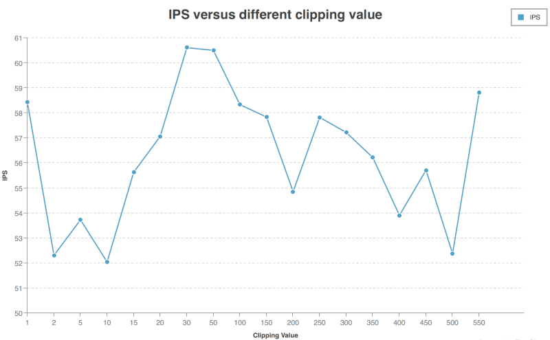
IPS Curve:

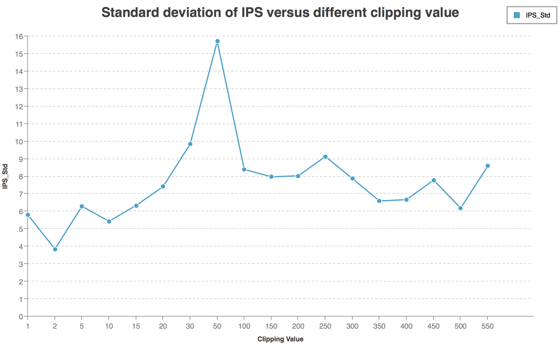
IPS-Std Curve:

Discussions

Not coincidence

I notice that when \(30<c<50\), the IPS is the highest (over \(60\)). However, the standard deviation is also quite high (over \(10\)). I train the network again when \(c=50\), the IPS is still over \(60\). So I think the local peak when \(30<c<50\) is not a coincidence.

Why standard deviation is so high?

In the evaluation process, IPS is calculated by

\[ \frac{10^4}{n^+ + 10n^-}\sum\delta\frac{\frac{score(\hat{x})}{\sum score(x_i)}}{\pi_0} \]

In another word, we calculate \(\pi_w=\frac{score(\hat{x})}{\sum score(x_i)}\).

Assume the output of our network is \(\sigma\), then score is calculated by \(score=e^{score-\max(score)}\) in the evaluation program.

The standard deviation is measured by

\[ \frac{2.58\times \sqrt{n}}{n^+ + 10n^-}\times Stderr[\delta \frac{\frac{ score(\hat{x})}{\sum score(x_i)}}{\pi_0}] \]

Note that we apply a post-process trick that \(\sigma' = \frac{850100}{1+e^{-\sigma +1.1875}}\).

Before post-process \(\sigma\):

896678244; 0:0.011302, 1:0.00727101, 2:0.0111319, 3:0.000752336, 4:0.00235881, 5:0.0131616, 6:0.00344201, 7:0.0268872, 8:0.0108119, 9:0.022044, 10:0.0268872

After post-process \(\sigma'\):

896678244; 0:200400, 1:199783, 2:200374, 3:198788, 4:199033, 5:200685, 6:199198, 7:202811, 8:200325, 9:202049, 10:202796

Before post-process \(\pi_w=\frac{score(\hat{x})}{\sum score(x_i)}\):

896678244; 0:0.984536, 1:0.980575, 2:0.984368, 3:0.974204, 4:0.97577, 5:0.986368, 6:0.976827, 7:1, 8:0.984053, 9:0.995168, 10:1

After post-process \(\pi_w=\frac{score(\hat{x})}{\sum score(x_i)}\):

896678244; 0:0, 1:0, 2:0, 3:0, 4:0, 5:0, 6:0, 7:1, 8:0, 9:0, 10:3.05902e-07

So actually our post-processing makes the policy more strict. For example, as shown above, after post-processing, id=896678244 gets a propensity vector \([0, 0, 0, 0, 0, 0, 0, 1, 0, 0, 3.05902e-07]\). So, if 7 is not the selected candidate, \(\pi_w\) will be \(0\), else \(\pi_w\) will be \(1\).

If not post-process, the propensity vector will be \([0.985, 0.981, 0.974, 0.976, 0.986, 0.977, 1, 0.984, 0.995, 1]\). Then \(\pi_w\) will be almost \(\frac{1}{11}\) no matter which candidate is selected.

So it’s easy to understand after post-processing, standard deviation will be much higher.

And it clear that post-processing is necessary. Because if not, the expectation of \(\pi_w\) will always be close to \(\frac{1}{11}\), no matter how nice the model is.

I think this is a BUG of the evaluation program. It should not use \(score=e^{score-\max(score)}\) but something like \(score=e^{\frac{score-\max(score)}{\sum score}}\).

Question: Why Standard deviation varies with clipping value? Why higher IPS often accompanies with higher Standard deviation?

Review what I am doing

What I am doing is training a network \(\sigma\) to minimize the loss function (If clipping is applied)

\[ -\min\{\frac{1}{p}, c\}\left[ y \cdot \log \sigma(x) + (1 - y) \cdot \log (1 - \sigma(x)) \right], \]

An important point is that \(y\) is whether this Ad is clicked, instead of whether this Ad is chosen to display. This is the difference between banditNet and my net.

Then, we use our network \(\sigma_{\bar{w}}\) to estimate the probability of clicking of a given Ad, and use this propensity as the propensity to display this Ad.

This is based on an assumption that \(\pi_0\) will always choose Ads with high CTR (reward) to display.

If this assumption is true (of course true), then the IPS:

\[ IPS = \frac{10^4}{n^+ + 10n^-}\sum\delta\frac{\frac{score(\hat{x})}{\sum score(x_i)}}{\pi_0} \]

will be maximized. This is how my net works.

Question: Why do we need to add \(\min\{\frac{1}{p}, c\}\) before our BCE loss fuction? Why will this contribute to CTR prediction?

In the banditNet settings, the network will directly calculate propensity for each candidate, or \(\pi_w\), then directly maximize the IPS / SNIPS or minimize its Lagrangian.

\[ IPS = \frac{1}{n}\sum\delta\frac{\pi_w}{\pi_0} \]

What’s the best clipping value?

According to the diagram drawn in the beginning, the best clipping value is around \(30\) ~ \(50\). The percentage of clipped propensities are about \(30\%\) ~ \(45\%\).

Question: Will \(30\%\) ~ \(45\%\) always be the best percentage? How to find the relationship between the best clipping value and the distribution of propensity?

Question: Is it true that the more propensities are clipped, the larger bias is and the smaller variance is? What’s the relation between bias-variance-tradeoff and clipping method?

Question: Is there better way to find the best clipping value without grid search?